time-series-forecasting
Links
Table of Contents
- Bikes for thee, not for me
- The world of data science
- Integrating data
- Synthesizing data
- Visualizing data
- Transforming data
- Sampling data
- Predicting data
- Bikes for thee, and for me
Bikes for thee, not for me
Bikes are great. On sunny days, I love riding while enjoying a cool breeze. And with bike stations scattered all around the city, I can just stroll towards the closest one for some daily errands.
Or so I thought…
![]()
The station is empty. I should have gotten there sooner. Or should I? Maybe if I wait a while, a bike will come to me? Could I predict when the bike station will run out of bikes?
Unfortunately, I’ve been confronted with this issue enough times that I started framing it as a data science problem (instead of buying my own bike). My first instinct was to look for some data to leverage for a divination session:
If you too are frustrated at the prospect of getting stranded in an empty bike station, tag along, I’ve got a ride for you. A ride into…
…The world of data science
A powerful tool to extract actionable insights from data. In our case, using data archives of hourly weather records and times of trips between bike stations, we’ll attempt to answer this question: “Given the weather, the location of the bike station, and the number of bikes in the station, how many bikes will be available in the future?”
Our journey will take us through these steps:
- Integrating data
- Synthesizing data
- Visualizing data
- Transforming data
- Sampling data
- Predicting data
In each section I’ll mention what is being done and why it’s being done. If you are interested in how things are done, check out the code in the source files. Each file corresponds to a section, and can easily be read along. If you’d like to reproduce the results, you’ll need data from the links above, a working installation of sqlite, and the following python packages:
python3 -m pip install contextily geopandas haversine numba plotly pytorch seaborn tqdm
1. Integrating data
To bake a cake, you need processed ingredients. You wouldn’t just toss raw wheat and cocoa beans in the oven and call it a day. You need to refine them first. And it’s the same for data science. In this section, we’ll refine and combine our raw data to make it palatable.
Processing the weather
The weather file has one row per hour with various measurements. We parse it to select columns, fill missing values and format the datetime.
| datetime | temperature (°C) | humidity (%) | cloudiness (%) | wind speed (m/s) | rain (mm/h) | snow (mm/h) |
|---|---|---|---|---|---|---|
| 2015-05-10 08:00:00 | 8.3 | 89 | 90 | 4.1 | 0.3 | 0 |
| 2015-05-10 09:00:00 | 8.25 | 92 | 90 | 3.1 | 0 | 0 |
| 2015-05-10 10:00:00 | 8.01 | 92 | 90 | 4.1 | 0 | 0 |
| 2015-05-10 11:00:00 | 7.75 | 96 | 90 | 4.1 | 0.3 | 0 |
| 2015-05-10 12:00:00 | 7.78 | 96 | 90 | 5.1 | 2 | 0 |
Processing stations
Each file is a snapshot of different stations, with their coordinates, name, and maximum capacity.
| id | name | latitude | longitude | capacity |
|---|---|---|---|---|
| 119 | Ashland Ave & Lake St | 41.88541 | -87.66732 | 19 |
| 120 | Wentworth Ave & Archer Ave | 41.854564 | -87.631937 | 15 |
| 121 | Blackstone Ave & Hyde Park Blvd | 41.802562 | -87.590368 | 15 |
| 122 | Ogden Ave & Congress Pkwy | 41.87501 | -87.67328 | 15 |
| 123 | California Ave & Milwaukee Ave | 41.922695 | -87.697153 | 15 |
Unfortunately, there are inconsistencies between snapshots. Some station properties change across time! Upon further investigation, we observe:
- Between two snapshot dates, a same station id can have different names.
- Between two snapshot dates, a same station id can have different capacities.
- Between two snapshot dates, a same station id can be over 90 meters apart.
- At any given snapshot date, all stations are more than 90 meters apart.
- At any given snapshot date, all stations have a unique station id.
To solve this, we assume that stations at most 90 meters apart with a same id and capacity are the same station, and all other stations are different stations. We assign proxy coordinates to each station, which are its average coordinates across all snapshot dates. This gives us a more consistent table.
| snapshot id | station id | name | capacity | proxy latitude | proxy longitude |
|---|---|---|---|---|---|
| 887 | 119 | Ashland Ave & Lake St | 19 | 41.88541 | -87.66732 |
| 896 | 120 | Wentworth Ave & Archer Ave | 15 | 41.854564 | -87.631937 |
| 905 | 121 | Blackstone Ave & Hyde Park Blvd | 15 | 41.802562 | -87.590368 |
| 914 | 122 | Ogden Ave & Congress Pkwy | 15 | 41.87501 | -87.67328 |
| 923 | 123 | California Ave & Milwaukee Ave | 15 | 41.922695 | -87.697153 |
Processing trips
Each file is a quarterly report of bike trips. A row is a record of source/destination stations and departure/arrival times.
| start datetime | stop datetime | start station id | start station name | stop station id | stop station name |
|---|---|---|---|---|---|
| 5/10/2015 9:25 | 5/10/2015 9:34 | 419 | Lake Park Ave & 53rd St | 423 | University Ave & 57th St |
| 5/10/2015 9:24 | 5/10/2015 9:26 | 128 | Damen Ave & Chicago Ave | 214 | Damen Ave & Grand Ave |
| 5/10/2015 9:27 | 5/10/2015 9:43 | 210 | Ashland Ave & Division St | 126 | Clark St & North Ave |
| 5/10/2015 9:27 | 5/10/2015 9:35 | 13 | Wilton Ave & Diversey Pkwy | 327 | Sheffield Ave & Webster Ave |
| 5/10/2015 9:28 | 5/10/2015 9:37 | 226 | Racine Ave & Belmont Ave | 223 | Clifton Ave & Armitage Ave |
Since we want trips between two locations, we must merge them with the stations table. Unfortunately, station ids aren’t reliable over time, so we use three properties to accurately join trips and stations: the station id, the station name, and the date of the trip. This operation is implemented in SQL which is more efficient for complex merging. The result is a list of trip dates and station snapshots.
| start datetime | stop datetime | start station snapshot id | stop station snapshot id |
|---|---|---|---|
| 2015-05-10 09:25:00 | 2015-05-10 09:34:00 | 3199 | 3223 |
| 2015-05-10 09:24:00 | 2015-05-10 09:26:00 | 965 | 1673 |
| 2015-05-10 09:27:00 | 2015-05-10 09:43:00 | 1637 | 947 |
| 2015-05-10 09:27:00 | 2015-05-10 09:35:00 | 59 | 2651 |
| 2015-05-10 09:28:00 | 2015-05-10 09:37:00 | 1772 | 1745 |
2. Synthesizing data
We now have a coherent set of processed ingredients. But wait, something’s missing! Our question was: “Given the weather, the location of the bike station, and the number of bikes in the station, how many bikes will be available in the future?”
We have the weather and locations of bike stations, but we don’t have the number of bikes in each station. Is there a way to figure that out? Actually, we do have trips between stations, so we can infer the number of available bikes by summing arrivals and departures. We can also use each station’s maximum capacity as a ceiling for the sum of incoming and outgoing bikes.
This operation requires a loop to incrementally sum and ceil the number of available bikes. Using numba, the loop is compiled to run at native machine code speed. Finally, the missing piece is revealed.
| proxy id | datetime | available bikes |
|---|---|---|
| 217 | 2015-05-10 09:00:00 | 12 |
| 217 | 2015-05-10 10:00:00 | 11 |
| 217 | 2015-05-10 11:00:00 | 12 |
| 217 | 2015-05-10 12:00:00 | 13 |
| 217 | 2015-05-10 13:00:00 | 15 |
3. Visualizing data
Data are the pigments we use to paint a beautiful canvas conveying a story. So far, we’ve looked at our data in tabular format, with lonesome dimensions spread across columns. Let’s blend these dimensions together to get a comprehensive view of bike availability across space and time.
A good graph is self-explanatory, but for clarity’s sake, here’s a description of what we see. Each point is a bike station in Chicago. A point’s color changes with the percentage of bikes available in the station, green when the station is empty, and blue when the station is full. What’s remarkable is that we already clearly see a pattern! On weekdays, downtown gets filled with bikes, breathing in all the commuters in the morning, and sending them back home in the evening.
4. Transforming data
Remember our processed ingredients? This is the part where we whip the eggs and weigh the chocolate to gather primed and balanced amounts. Transforming and scaling are necessary to provide understandable and comparable data to our prediction model.
Let’s start by scaling the percentages of available bikes to a range between 0 and 1.
![]()
Next, we project station latitudes and longitudes to Cartesian coordinates and normalize them. We also compute the distance of each station to the city center and scale that.
![]()
What is 3 - 23? If you say -20 you are technically correct, but semantically wrong. When comparing times, 3 and 23 are just 4 hours apart! Unfortunately, a machine only understands technicalities. So how do we connect times at midnight? We transform hours into cyclical features that continuously oscillate between -1 and 1. To tell all the hours apart, we use both sine and cosine transformations, so every hour has a unique pair of mappings.
![]()
We also scale temperature, humidity, cloudiness, wind speed, rain, and snow, so they all lie approximately in the same range between 0 and 1.
![]()
From those distributions we notice that many rain and snow measurements equal 0. Our dataset seems skewed. When training our model, we must make sure to give it enough cases of rainy and snowy days so it learns to pay attention to those features.
5. Sampling data
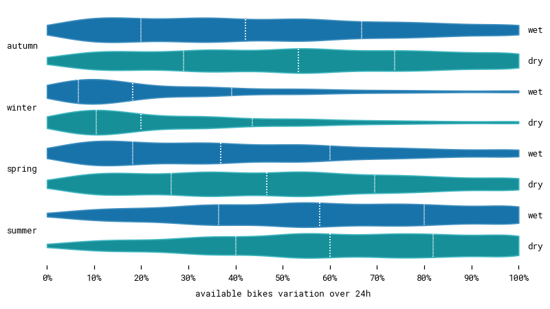
One way to obtain a homogenous dataset is to sample it to select enough measurements in each category. First let’s see how our data is distributed. We segment it into overlapping 24 hour sequences that will be used to train our model.
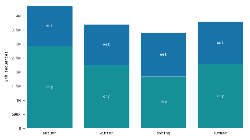
We have different numbers of sequences in each season and there are less wet days than dry days. However, the differences aren’t extreme. We still have lots of data in each category, which should be enough to train our model. Notice that while there are very few actual hours with rain or snow, there are considerably more wet sequences with some amount of precipitation. Viewing data is a matter of perspective.
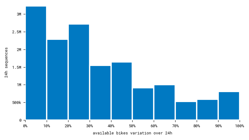
Bike availability is the target feature we want to predict. Unfortunately, many bike stations keep the same number of bikes over long periods of time. That means there’s a risk our model will predict an unvarying number of bikes, whatever the input sequence! To avoid this, we must select a uniform subset of data including enough cases of stations that are often visited throughout the day.
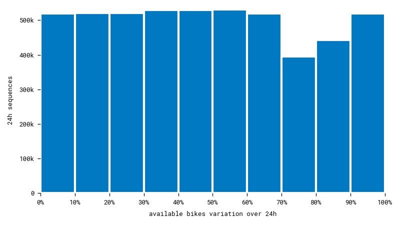
After sampling at random within each interval, we get a much more uniform dataset. Having plenty of different cases will help the model learn better.
Going deeper, we can cross seasons and variation to determine how they are correlated. Unsurprisingly, we observe less variation in winter when it’s cold. And even less on wet days when it’s snowing. After all, there aren’t many bike stations getting visited in a blizzard in the middle of December. Can our model understand that to make more accurate predictions?
6. Predicting data
Now that all our ingredients are ready, we can move on to the next step: baking our model. What kind of model do we want? One that can predict time series of bike availability from other sequences. Let’s find a mold for that.
Choosing the model architecture
For a neural network, there are several different architectures suitable for sequence prediction. Our main contenders are:
- The recurrent neural network (RNN)
- The long short-term memory network (LSTM)
- The transformer
Here’s a quick and basic overview of each architecture.
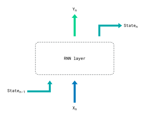
A RNN is a model that updates its state recursively at each sequence step, by taking into account its previous state and the current sequence item. Recurrent neural networks suffer from long-term memory loss because they continuously focus on the last provided inputs, which eventually override longer dependencies. Basically, you can see a RNN as a goldfish that constantly rediscovers its environment.
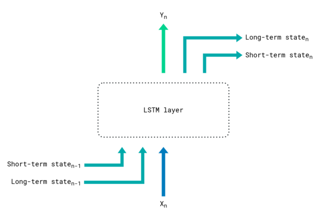
A solution to long-term memory loss is the LSTM, which is a RNN upgraded with two internal states: a short-term state that grasps the most recent developments, and a long-term state that can ignore sequence items as they are encountered. It’s still a goldfish, but now it keeps a diary. This helps preserve long-term dependencies, but stays computationally expensive as the sequence must be processed recursively.
![]()
Enters the transformer, a state-of-the-art architecture for sequence processing and prediction. It solves both long-term memory loss and computational cost by eliminating recursion during training. Each sequence item is appended to a positional encoding that enables processing the entire sequence as a whole. This is all done in parallel with multiple attention heads, each one trained to understand a specific relationship between sequence items. Like a school of cognitively-enhanced, higher-dimensional goldfish, processing all time-bound events at once.
In the original paper introducing the transformer [1], the architecture is used for machine translation between languages. In other words, it maps one sequence to another sequence. This seems promising for our use case, except that we don’t have just one, but multiple sequences for bike availability and weather, in addition to some constants like station coordinates.
Looking for available implementations of the transformer architecture tweaked to work with multivariate data didn’t yield anything directly usable, but there is a paper that focuses on solving that for spatio-temporal forecasting [2]. They concatenate sequences together, along with variable embeddings, before inputting them to the network. They also introduce two new modules: global attention to examine relationships between all sequences mutually, and local attention to find relationships within each sequence individually. This seems to suit our needs, so let’s apply these concepts to build a fully functional model.
Implementing the model
Taking inspiration from the above sources and tuning them to simplify and generalize, the end result is an architecture similar to a vanilla transformer, but modified to accommodate multiple variables with the following enhancements:
- An additional dimension to separate variables in attention modules.
- Different modules for local and global attention among variables.
This way, we can avoid concatenating sequences in one big matrix along with variable embeddings. Every variable is processed individually, except when they are pitched against each other in the global attention modules.
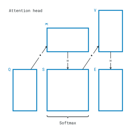
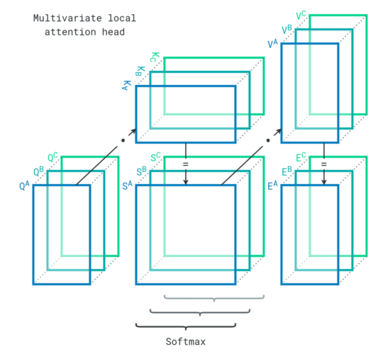
To explain further, here is how an attention head works. First, the sequence is projected into query (Q), key (K), and value (V) matrices. Each row corresponds to a sequence item. Query and key matrices are then multiplied to yield a score (S) matrix, where each row is softmaxed to emphasize the strongest relationships between sequence items. The score matrix is then multiplied with the value matrix to yield an encoding (E) of the original sequence.
In our case, we have multiple variables, so each attention head gets an additional dimension to accommodate the sequences. The operations are the same as in the original transformer, but parallelized for multiple variables (A, B, C). This is how an attention head behaves in our local attention module.
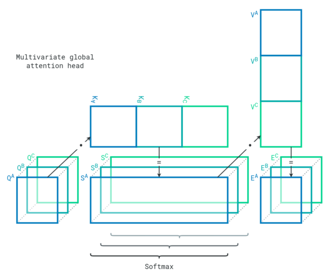
Local attention modules learn relationships within each sequence, but the model must also figure out relationships between sequences. To do so, attention heads can concatenate key projections and value projections to reduce their number of dimensions. This effectively allows each sequence item to encounter every other sequence item of every variable. The strengths of their relationships are directly available in the score matrices. This is how an attention head behaves in our global attention module.
Training the model
The architecture is implemented but the model is completely ignorant at this point. It hasn’t seen any data, it doesn’t know anything about the world. The next step is to train it with a part of the dataset that we call the training-and-validation set. The training-and-validation set is like a collection of corrected exam papers with questions and answers. In our case, the “questions” are the number of bikes, weather, and location, and the “answers” are the future number of bikes. The goal of training is to teach the model to get the correct answers to questions. Like a student studying diligently by practicing on past exams every day, the entire training-and-validation set is provided to the model at every epoch:
- First, the collection of exam questions are split into a large training set and small validation set.
- The model reads some questions from the training set and attempts to answer them.
- The model mentally adjusts its knowledge depending on how well it answered.
- Repeat steps 2 and 3 until the entire training set has been seen.
- The model takes a mock exam on the validation set and attempts to answer without peeking.
- The model’s answers on the mock exam provide an estimate of its performance.
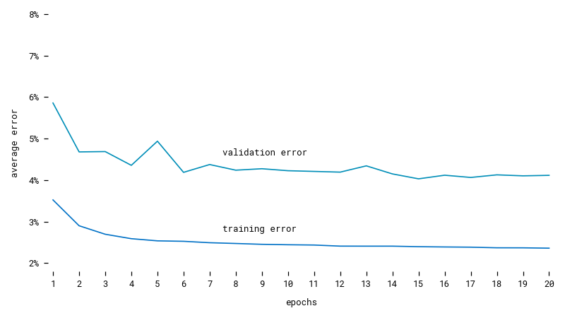
Training our model on a subset of data to predict the next 6 hours from the previous 18 hours shows that it learns and stabilizes rather quickly. Even though the training-and-validation set is shuffled at each epoch, the validation error stays above the training error. That’s because recursion is eliminated during training, so for each hour to predict, the model sees the entire sequence that comes before, but during validation, the model only sees the input sequence and has to predict all the following hours on its own.
After the model has trained enough times, it is deemed ready to take the final exam on the testing set. The testing set is the other part of the dataset that the model has not yet encountered. This exam really measures the intelligence of the model. If it learned the answers of past exams by heart, it will fail on new unseen questions. But if it correctly understood relationships between questions and answers, it will be competent enough to generalize to novel cases. The model passes the test with an average error of around 4%, or about 1 bike of error in a station of 25 bikes. Not bad at all! Check out some of its predictions below.
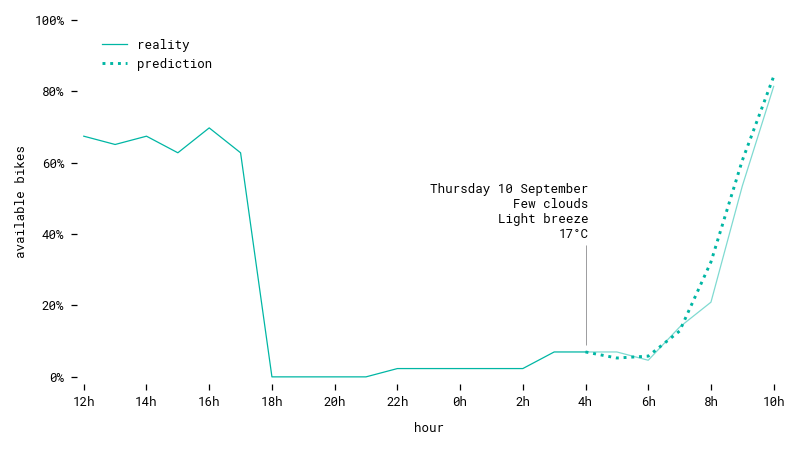
Prediction for a station on a workday in autumn. The model understands this station is highly visited in the morning, and predicts a trend accordingly.
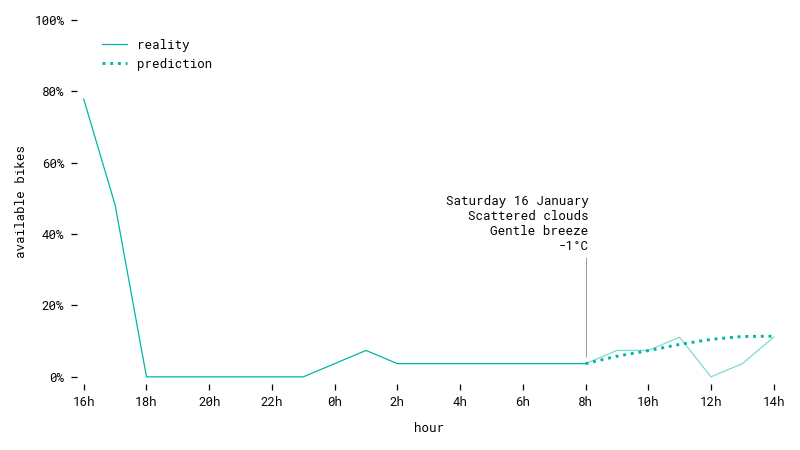
Prediction for a station during a winter weekend. The model successfully guesses a slight upward trend throughout the day.
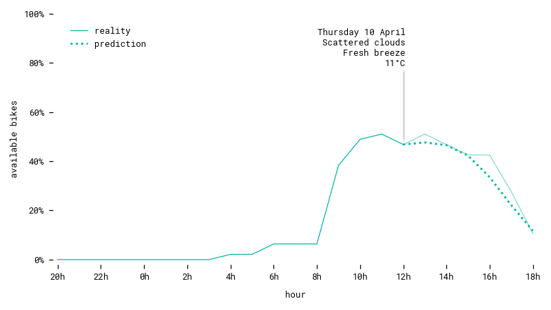
Prediction for a workday in spring. The prognostic is a downward trend during the afternoon, which comes true.
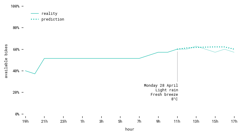
Another prediction for a workday in spring, with some amount of rain. The model accurately predicts little variation for this station.
Bikes for thee, and for me
This concludes our journey through the realms of data science. Transformers work really well for sequence generation. If you’re interested in reading more about that, check out the references below.
- Vaswani et al. (2017) Attention Is All You Need
- Grigsby et al. (2021) Long-Range Transformers for Dynamic Spatiotemporal Forecasting